Project Overview
Shiyu Huang, Hongxiang Qiu, Zeyu Zhao, Zongren Zou
In this project, we parallelized an algorithm called DeepFlow with multiple techniques (MPI, OpenMP and OpenACC). Since DeepFlow is useful not only on image processing but also on video processing where independent flows can be generated simultaneously, we thus applied MapReduce for the video processing tasks. Our test result shows the parallelized DeepFlow algorithm can run faster on both image tasks and video tasks.
Below are the links to the required contents (in grading rubric):
- Application design: profiling and parallelization design
- Problem solution: introduction of the problem (optical flow and DeepFlow) and need for HPC. Parallelization is not trivial due to serial dependencies and we changed the algorithm
- Implementation approach: Parallelization implementations and corresponding code. Data can be any two consecutive images or videos. See data preparation and sample data here
- Platform deployment: evaluation platform. Guide to deploy on AWS (or other systems): GitHub README
- Application software: different parallelizations and applications of DeepFlow (application examples)
- Software documentation: GitHub README. There're some separate READMEs for specific modules. You can access them via the links in the main README.
- Performance evaluation and discussion: performance of different linear solvers and different parallelizations (also see overhead analysis and optimizations in the implementation section)
- Advanced features: RBSOR and application on slow motion video generation
Optical Flow
Optical flow computation is a key component in many computer vision systems designed for tasks such as action detection or activity recognition. It has many important applications in computer vision, including slow motion video generation, object tracking and etc. Starting from the famous Horn-Schunck algorithm (B. K. Horn and B. G. Schunck. Determining optical flow. Proc. SPIE 0281, Techniques and Applications of Image Understanding, 1981.) and Lucas-Kanade algorithm (B. D. Lucas and T. Kanade. An iterative image registration technique with an application to stereo vision. In IJCAI, volume 81, pages 674–679, 1981), researchers have conducted decades of pioneering research, achieving great development in this area.
Below is a visualization of optical flow. The left GIF is two consecutive frames in a video and the right picture is the visualization of the computed optical flow. (source: https://people.csail.mit.edu/celiu/OpticalFlow/)
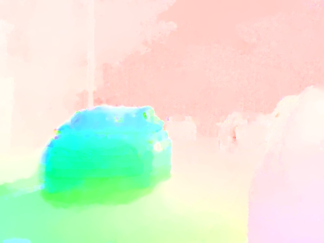
Optical flow algorithm aims at computing pattern of apparent motion of objects. Given two consecutive images, we would like to compute how each pixel moves from the first image to the second image. Imagine there are three-dimensional vectors describing the motion of the objects in 3-D space. Ideally, the optical flow is the 2-D projection of the three-dimensional vectors on the image. In computer vision, we call this projected two-dimensional vector as flow field. There are four important assumptions for optical flow algorithm:
- Brightness constancy: The image grey value of the pixel does not change during the motion.
- Gradient constancy: it is useful to allow some small variations in the brightness because it often appears in natural scenes. So we assume that the gradient of the image grey value does not vary due to the displacement.
- Smoothness: The movement is a smooth movement.
- Small displacement: Between each pair of consecutive images, the corresponding pixels do not move too far.
- Spatial coherence: points move like their neighbors within patches.
Most optical flow algorithms develop their ideas on the basis of these assumptions.
DeepFlow
There're many algorithms for optical flow estimation, each with its own focus of special optimization in some aspects. One of the state-of-the-art algorithm is the DeepFlow algorithm. This algorithm has its focus on solving large displacement in optical flow estimation. This property makes it ideal for slow motion video applications (in the scenario of generating slow motion videos, the original videos are likely to have large displacement between consecutive frames). Although there're some real-time optical flow estimation algorithms, their accuracy is worse compared to DeepFlow.
The deep flow algorithm mainly has two steps:
DeepMatching
The matching algorithm is used to compute the matching of corresponding pixels in consecutive frames. The deep matching algorithm is built upon a multi-stage architecture with about 6 layers (depending on the image size), interleaving convolutions and max-pooling (a structure similar to deep convolutional nets). The matching stage is to prepare for the flow computation stage.
The deep matching code is already parallelized and we will just use the existing implementation in our project. Therefore we will skip further explanations on this part.
DeepFlow
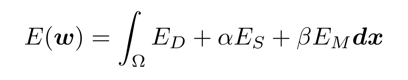
Deep flow is a variational refinement method that blends the result from deep matching algorithm into an energy minimization framework. The energy that the algorithm minimizes (equation below) is a weighted sum of data term ED, smoothness term Es and matching term EM.
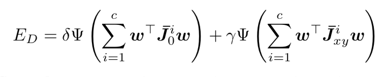
ED is a combination of separate penalization of the color and gradient constancy assumptions with a normalization factor.
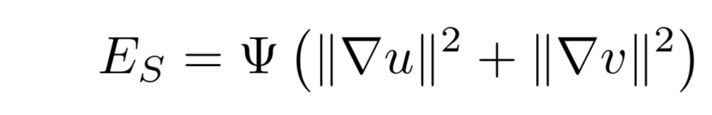
Es is based on the smoothness assumption. It is a robust penalization of the gradient flow norm.
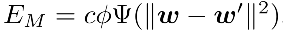
EM penalizes the difference between the flow and the pre-computed matching vector from deep matching.

Obviously, the energy function is non-convex and non-linear and it contains integrals, so that energy minimization is pretty complicated. Fortunately, energy function with integrals inside can be minimized by solving its Euler-Lagrange equations, which are second-order partial differential equations, and can be easily derived from integrals in energy function. This is called variational approach, and the solutions are actually functions instead of vectors in regular optimization problems, which fits our optical flow problem perfectly. However, the Euler-Lagrange equations are still nonlinear, and to approximate them with linear system so that they are tractable and can be solved with common numerical methods, we first need to apply fixed point iterations and downsampling and then use first order Taylor expansions to finally get our linear approximation. Furthermore, in order to solve the linear system, we still need numerical methods to have both stable and accurate solution. There are numerous numerical methods for linear system. The original implementation uses Successive Over Relaxation (SOR) method to solve the linear system.
Need for HPC and Big Data
Using DeepFlow (default settings) to calculate the flow of two 1080p images takes 43 seconds. The time cost is expected to increase linearly as the image size increases, which means 11 minutes for two 8K images. In addition, optical flow is often applied to image sequences (i.e. video). For a 25fps 1080p video, if we want to calculate both forward and backward flows, we need to run DeepFlow 50 times per 1 second video length on average and this means processing 1 second video takes around 36 minutes on a single CPU. If we have a 1080p video of 20 minutes in length, generating the flow on a single CPU takes a month. There're significantly faster algorithms like Dense Inverse Search (DIS), but the accuracy is also worse. For some tasks (like slow motion video generation), we may need good accuracy.
By using HPC techniques, we can reduce the running time for every single flow. By using Big Data techniques, we can generate multiple flows simultaneously. Therefore, with HPC and Big Data, we can significantly reduce the running time of DeepFlow and make it realistic to apply DeepFlow on long videos.
Challenges
- The DeepFlow algorithm is not easy to understand.
- Most of time is spent on linear system solver. However, the current linear system solver is not parallelizable due to serial dependency.
- For MPI, the message exchange is not trivial.
- It's pretty hard to apply MapReduce in our problem because the code is in C and the data is binary. (So we can't trivially use Hadoop Streaming like in assignment).
- We want to show some applications of DeepFlow on videos so our work is meaningful. This is not always easy (for example there's existing code but it does not use DeepFlow to calculate the optical flow and we have to write some code to let it use DeepFlow).